NumPy and Linear Algebra

This article is mostly about how to use the Python module, NumPy, for matrix calculation and is written as a reference for the one who takes or will take EECS 16A at Berkeley.

What is NumPy?

NumPy is the library for scientific computation. According to the official website,

NumPy is the fundamental package for scientific computing in Python. It is a Python library that provides a multidimensional array object, various derived objects (such as masked arrays and matrices), and an assortment of routines for fast operations on arrays, including mathematical, logical, shape manipulation, sorting, selecting, I/O, discrete Fourier transforms, basic linear algebra, basic statistical operations, random simulation and much more.

How to import NumPy

To start off the Numpy journey, we need to import NumPy first. The code below imports the NumPy library as the name of np.

# install NumPy and named 'np'
import numpy as np

Creating NumPy Array Object

NumPy array object is very similar to the Python List (reference to List). However, unlike Python List, some method does not support NumPy (e.g. sort() and reverse()). In Numpy, both vector and matrix are stored in ndarray (※ short for N dimensional array). However, utilizing cast, you can either the Python List method or NumPy method. There are multiple ways to create the matrix with NumPy.

Example 1 (Creating matrix with`array()`)

Create the iterable object and plug it into NumPy Array with array().

array() reference

# normal Python List
list = [1, 2, 3, 4, 5]
# normal Python Tuple
tup = ((1, 2, 3, 4, 5), (6, 7, 8, 9, 10))

# NumPy Array object
mtx1 = np.array(list)
mtx2 = np.array(tup)

print("list :\n", list)
print("mtx1 :\n", mtx1)

print("tup :\n", tup)
print("mtx2 :\n", mtx2)

# output
list :
 [1, 2, 3, 4, 5]
mtx1 :
 [1 2 3 4 5]
tup :
 ((1, 2, 3, 4, 5), (6, 7, 8, 9, 10))
mtx2 :
 [[ 1  2  3  4  5]
 [ 6  7  8  9 10]]

Example 2 (Plugging in Each Component with `empty()`)

By using empty([<SIZE OF ROW>, <SIZE OF COLMN>]), you can create the empty NumPy array, and also using dtype keyword, you can restrict the data type. However, the array created by empty() sets totally random numbers in itself, you need to initialize it.

empty() reference

mtx = np.empty([3,3])
for i in range(3):
    for j in range(3):
        mtx[i, j] = i + j # initializing Numpy Array.

print("mtx: \n", mtx)

mtx: 
 [[0. 1. 2.]
 [1. 2. 3.]
 [2. 3. 4.]]

Example3 (identity array `eye()` and array with all zeros `zeros()`)

In some cases, there is a much simpler way to create an array. For example, to create an identity array, a square matrix which diagonal element are 1 and the others are 0, in which all diagonal elements are 1, eye() is much simpler than creating the array and initializing all of the elements with 1 diagonally. Also, zero vector or zero matrix, the vector or matrix in which all components are zero, can be created using zeros()

Example of identity matrix 3 by 3

$np.eye{\textbf{}}(3)=\begin{pmatrix} 1& 0 & 0 \\ 0& 1 & 0 \\ 0& 0 & 1 \\\end{pmatrix}$

Example of zero matrix 3 by 3 $np.zeros([3,3]) = \begin{pmatrix}0 & 0 & 0 \\0 & 0 & 0 \\0 & 0 & 0 \\\end{pmatrix}$

eye() reference
zeros() reference

# to create identity matrix
identity_mtx = np.eye(5)
print("identity matrix\n", identity_mtx)

# to create zeros matrix
zero_mtx = np.zeros([5,5])
print("zeros matrix\n",zero_mtx)

# output
identity matrix
 [[1. 0. 0. 0. 0.]
 [0. 1. 0. 0. 0.]
 [0. 0. 1. 0. 0.]
 [0. 0. 0. 1. 0.]
 [0. 0. 0. 0. 1.]]
zeros matrix
 [[0. 0. 0. 0. 0.]
 [0. 0. 0. 0. 0.]
 [0. 0. 0. 0. 0.]
 [0. 0. 0. 0. 0.]
 [0. 0. 0. 0. 0.]]

Broadcasting Arithmetic manipulation on NumPy Array

By using NumPy module, you do not need to calculate the matrix by hand anymore.

import numpy as np
mtx = np.array([[1,1,1], [1,1,1], [1,1,1], [1,1,1]])

print("mtx\n", mtx)

print("mtx1 + 10\n", mtx + 10) # addtion
print("mtx2 - 1\n", mtx - 1) # substitution
print("mtx1 * 10\n", mtx * 10) # multiplication
print("mtx2 / 10\n", mtx / 10) # division

# output
mtx
 [[1 1 1]
 [1 1 1]
 [1 1 1]
 [1 1 1]]
mtx1 + 10
 [[11 11 11]
 [11 11 11]
 [11 11 11]
 [11 11 11]]
mtx2 - 1
 [[0 0 0]
 [0 0 0]
 [0 0 0]
 [0 0 0]]
mtx1 * 10
 [[10 10 10]
 [10 10 10]
 [10 10 10]
 [10 10 10]]
mtx2 / 10
 [[0.1 0.1 0.1]
 [0.1 0.1 0.1]
 [0.1 0.1 0.1]
 [0.1 0.1 0.1]]

Accessing the Elements of NumPy Array

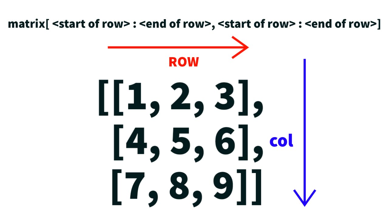
Always remind in your mind that the array index starts with 0, and the end of the row or col is not included.

Example of Accessing the Elements of NumPy Array

import numpy as np

mtx = np.array([[1, 2, 3],
                [4, 5, 6],
                [7, 8, 9]])

print("original matrix\n", mtx)

# Accessing the first row
print("Accessing the first row\n", mtx[0])
# Accessing the second col
print("Accessing the second col\n", mtx[:,1])
# Accesing the element at 2nd col and 2nd row
print("Accesing the element at 2nd col and 2nd row\n", mtx[1, 1])
# Accessing the matrix at 1-2 col and 1-2 row
print("Accessing the matrix at 1-2 col and 1-2 row\n", mtx[:2, :2]) 
# becareful the end of col or row is not included

# output
original matrix
 [[1 2 3]
 [4 5 6]
 [7 8 9]]
Accessing the first row
 [1 2 3]
Accessing the second col
 [2 5 8]
Accesing the element at 2nd col and 2nd row
 5
Accessing the matrix at 1-2 col and 1-2 row
 [[1 2]
 [4 5]]

Dot Product (Inner Product)

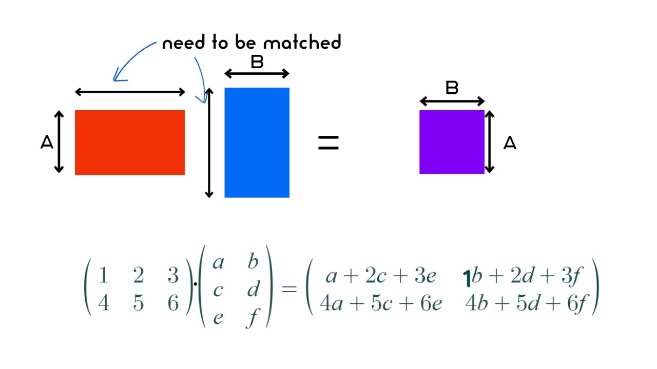
By utilizing np.dot(), the tiresome dot product of matrices can be easily solved. However, to calculate the matrix, the inner dimensions must be matched.

Example of Dot Product of NumPy

The example below calculate the dot product of 3 by 2 array and 2 by 3 array.

$A = \begin{pmatrix}1 & 2 & 3 \\4 & 5 & 6 \\\end{pmatrix}B = \begin{pmatrix}1 & 2 \\3 & 4 \\5 & 6 \\\end{pmatrix}$

$A \cdot B = \begin{pmatrix} 1& 2 & 3 \\ 4& 5 & 6 \\\end{pmatrix} \cdot\begin{pmatrix}1 & 2 \\3 & 4 \\5 & 6 \\\end{pmatrix}= \begin{pmatrix} 1 \cdot 1 + 2\cdot3 + 3 \cdot 5& 1 \cdot 2 + 2\cdot 4 + 3 \cdot 6 \\ 4 \cdot 1 + 5\cdot3 + 6 \cdot 5& 4 \cdot 2 + 5\cdot 4 + 6 \cdot 6 \\\end{pmatrix}$

$= \begin{pmatrix}22 & 28 \\49 & 64 \\\end{pmatrix}$

import numpy as np

a = np.array([[1, 2, 3],[4, 5, 6]])
b = np.array([[1, 2],[3, 4],[5, 6]])

print('the dot product of a and b\n', np.dot(a, b))

# output
the dot product of a and b
 [[22 28]
 [49 64]]

Transpose

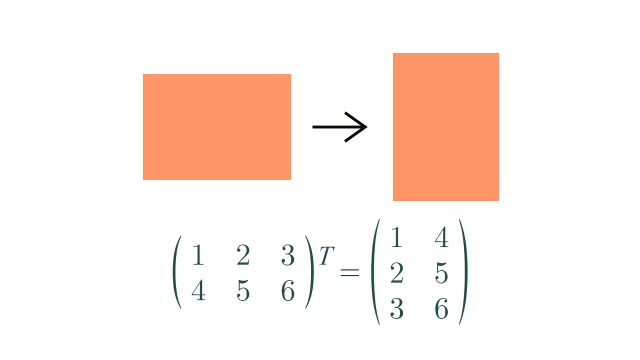
The matrix which switches rows and columns of the original matrix is called transpose of matrix. For example, the transpose of matrix m × n is n × m.

import numpy as np

mtx = np.array([[1, 2, 3], [4, 5, 6]])
print("original matrix\n", mtx)

transposed = np.transpose(mtx)

print("transposed matrix\n", transposed)

# output

original matrix
 [[1 2 3]
 [4 5 6]]
transposed matrix
 [[1 4]
 [2 5]
 [3 6]]

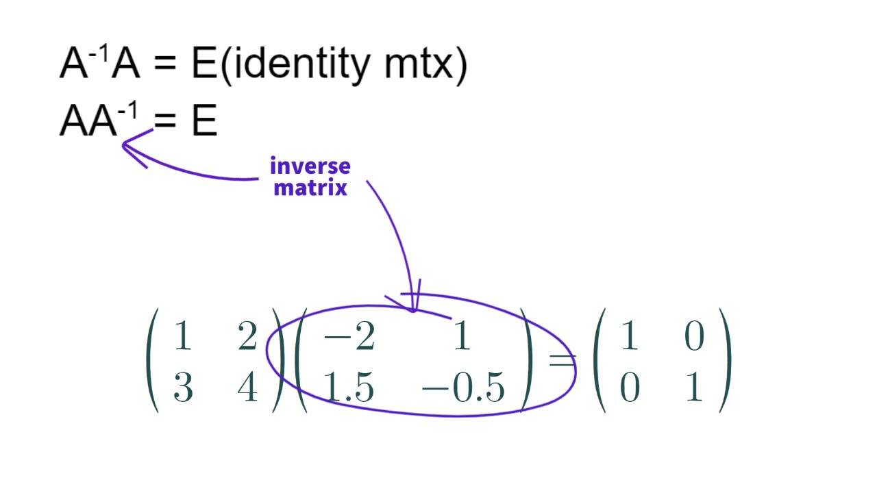
Inverse

The matrix in which col and row are the same is called square matrix. There is only one matrix such that the dot product of a certain square matrix and it is the identity matrix, and the matrix is called inverse matrix. Only linearly independent matrix has an inverse matrix of itself. Usually, finding the inverse of the matrix is really difficult using Gaussian-Jordan method. However, np.linalg.inv() facilitate the finding inverse of the matrix.

Example of Finding inverse matrix

The examples below find the inverse matrixes using Gaussian-Jordan method and np.linalg.inv()

Using Gaussian-Jordan method

import numpy as np

mtx = np.array([[1, 2], [3, 4]])

inversed = np.linalg.inv(mtx)

print("original matrix\n", mtx)

print("inverse matrix\n",inversed)

print("the dot product of the original matrix and inverse matrix\n",np.dot(mtx, inversed))

# output

original matrix
 [[1 2]
 [3 4]]
inverse matrix
 [[-2.   1. ]
 [ 1.5 -0.5]]
the dot product of the original matrix and inverse matrix
 [[1.0000000e+00 0.0000000e+00]
 [8.8817842e-16 1.0000000e+00]]

Conclusion

When I went to Community college, I took a linear algebra class and really had a difficult time calculating the voltage and current values on the circuit board. However, By using the Numpy library, the matrix calculation will be easier.